In this package, resampling is primary approach for optimizing predictive models with tuning parameters. To do this, many alternate versions of the training set are used to train the model and predict a hold-out set. This process is repeated many times to get performance estimates that generalize to new data sets. Each of the resampled data sets is independent of the others, so there is no formal requirement that the models must be run sequentially. If a computer with multiple processors or cores is available, the computations could be spread across these "workers" to increase the computational efficiency. caret leverages one of the parallel processing frameworks in R to do just this. The foreach package allows R code to be run either sequentially or in parallel using several different technologies, such as the multicore or Rmpi packages (see Schmidberger et al, 2009 for summaries and descriptions of the available options). There are several R packages that work with foreach to implement these techniques, such as doMC (for multicore) or doMPI (for Rmpi).
To tune a predictive model using multiple workers, the function syntax in the caret package functions (e.g. train, rfe or sbf) do not change. A separate function is used to "register" the parallel processing technique and specify the number of workers to use. For example, to use the multicore) package (not available on Windows) with five cores on the same machine, the package is loaded and them registered:
library(doMC)
registerDoMC(cores = 5)
## All subsequent models are then run in parallel
model <- train(y ~ ., data = training, method = "rf")
The syntax for other packages associated with foreach is very similar. Note that as the number of workers increases, the memory required also increase. For example, using five workers would keep a total of six versions of the data in memory. If the data are large or the computational model is demanding, performance can be affected if the amount of required memory exceeds the physical amount available. Also, for rfe and sbf, these functions may call train for some models. In this case, registering M workers will actually invoke M2 total processes.
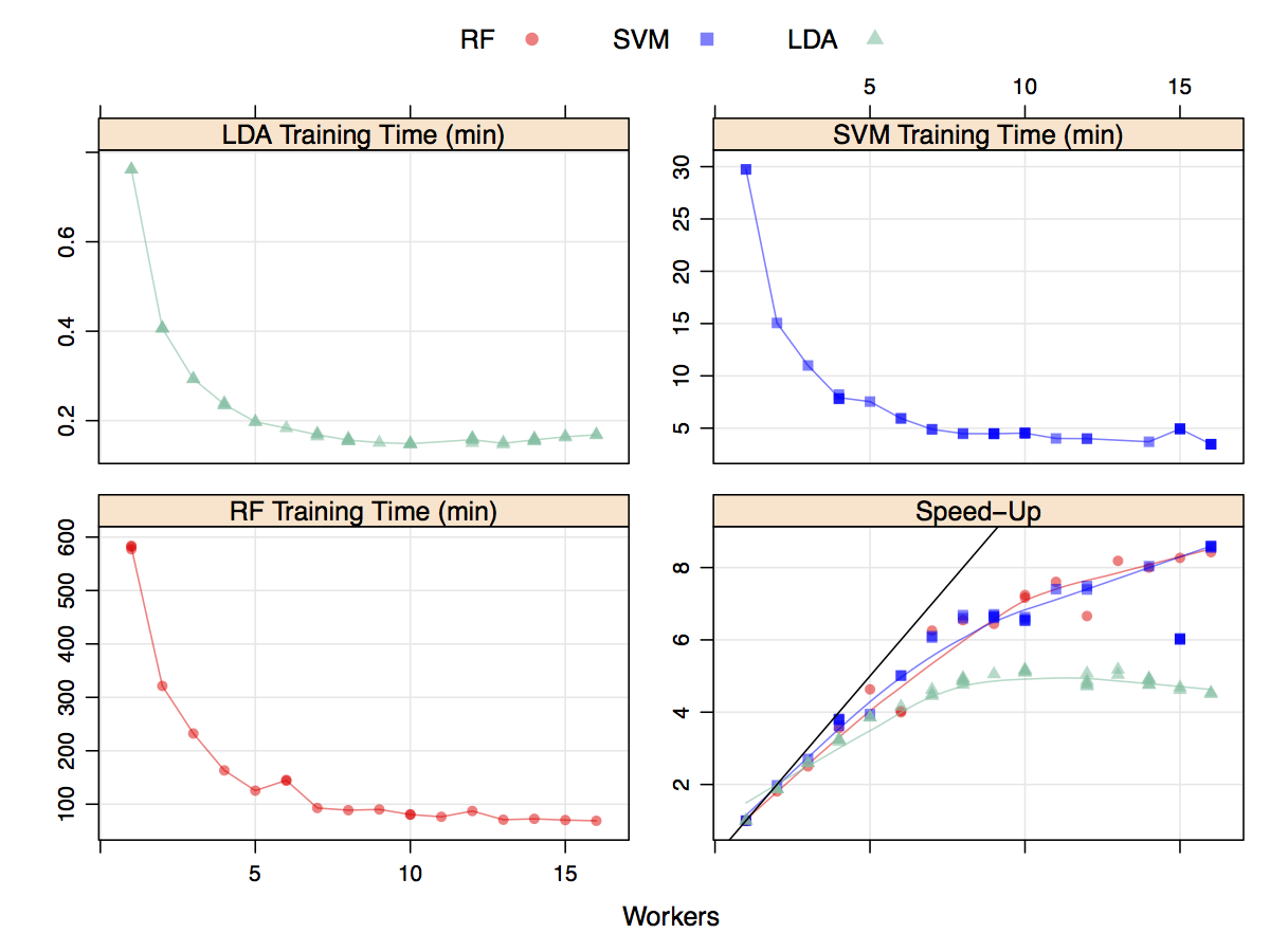
Does this help reduce the time to fit models? A moderately sized data set (4331 rows and 8) was modeled multiple times with different number of workers for several models. Random forest was used with 2000 trees and tuned over 10 values of mtry. Variable importance calculations were also conducted during each model fit. Linear discriminant analysis was also run, as was a cost-sensitive radial basis function support vector machine (tuned over 15 cost values). All models were tuned using five repeats of 10-fold cross-validation. The results are shown in the figure below. The y-axis corresponds to the total execution time (encompassing model tuning and the final model fit) versus the number of workers. Random forest clearly took the longest to train and the LDA models were very computationally efficient. The total time (in minutes) decreased as the number of workers increase but stabilized around seven workers. The data for this plot were generated in a randomized fashion so that there should be no bias in the run order. The bottom right panel shows the speed-up which is the sequential time divided by the parallel time. For example, a speed-up of three indicates that the parallel version was three times faster than the sequential version. At best, parallelization can achieve linear speed-ups; that is, for M workers, the parallel time is 1/M. For these models, the speed-up is close to linear until four or five workers are used. After this, there is a small improvement in performance. Since LDA is already computationally efficient, the speed-up levels off more rapidly than the other models. While not linear, the decrease in execution time is helpful - a nearly 10 hour model fit was decreased to about 90 minutes.
Note that some models, especially those using the RWeka package, may not be able to be run in parallel due to the underlying code structure.
train, rfe, sbf, bag and
avNNet were given an additional argument in their respective
control files called allowParallel that defaults to
TRUE. When TRUE, the code will be executed in parallel
if a parallel backend (e.g. doMC) is registered. When
allowParallel = FALSE, the parallel backend is always
ignored. The use case is when rfe or sbf calls
train. If a parallel backend with P processors is being used,
the combination of these functions will create P2 processes. Since
some operations benefit more from parallelization than others, the
user has the ability to concentrate computing resources for specific
functions.
One additional "trick" that train exploits to increase computational efficiency is to use sub-models; a single model fit can produce predictions for multiple tuning parameters. For example, in most implementations of boosted models, a model trained on B boosting iterations can produce predictions for models for iterations less than B. Suppose a gbm model was tuned over the following grid:
gbmGrid <-  expand.grid(.interaction.depth = c(1, 5, 9),
                        .n.trees = (1:15)*100,
                        .shrinkage = 0.1)
In reality, train only created objects for 3 models and derived the other predictions from these objects. This trick is used for the following models: bagEarth, blackboost, bstLs, bstSm, bstTree, C5.0, C5.0Cost, cubist, earth, enet, foba, gamboost, gbm, glmboost, glmnet, kernelpls, lars, lars2, lasso, lda2, leapBackward, leapForward, leapSeq, LogitBoost, pam, partDSA, pcr, PenalizedLDA, pls, relaxo, rpart, rpart2, rpartCost, simpls, superpc, widekernelpls.